About Me

Predicting Building’s Energy Use

Project Definition

Maintaining perfect indoor temperature in a skyscraper requires an extraordinary amount of energy which translates to money being spent to maintain those ideal conditions. Additionally, this energy expenditure may have negative impact on the environment. Fortunately, investments are being made to reduce cost and emissions. Buildings which install new and/or upgrade their existing equipment to more efficient ones can reduce energy consumption, cost, and environmental impact. However, how can these savings be measured?

“Under pay-for-performance financing, the building owner makes payments based on the difference between their real energy consumption and what they would have used without any retrofits. The latter values have to come from a model.” [1]

Additionally, how do we evaluate energy savings of the improvements? To do this, we need to estimate or model the amount of energy a building would have used before the improvements. After the improvements are made, we can compare the energy usage between the original building (modeled energy usage) and the retrofit building (actual energy usage). Then, these counterfactual models are used to calculate the energy savings due to the retrofit. [2]

The provided data was collected over a three-year period from over 1,000 buildings across the world. To capture true savings, the model must be quite robust and accurate. The ideal model will be able to find patterns which contribute to energy consumption. It must scale well since the training data includes over 20 million samples.

Problem Statement

The goal is to create a model which can predict a building’s energy use with minimal error. The first step is to use exploratory data analysis (EDA) to understand the nature of all present variables (continuous and discrete) using statistical plots, descriptive and inferential statistics. This exploration will help locate missing values, outliers, and relationships between variables. Ideally, the knowledge gained in this section will be leveraged to build a machine learning model that minimizes prediction error. Removing noisy data is important no matter which ML algorithm is used. Two potential algorithms will be evaluated, LightBGM and XGBoost. Both are tree-based algorithms and should perform well on this large data set.

Metrics

The model will aim to minimize the Root Mean Squared Log Error (RMSLE). It is defined as

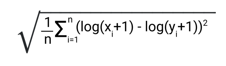
where Xi are the predicted values and Yi are the Actual values. Logarithmic properties let us rewrite this as

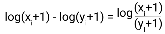
Essentially, the RMSLE gives us a ratio between the predicted and actual values. On the other hand, RMSE gives us an absolute value between the predicted and actual values. For example, if the predicted value is 1000 and actual is 500, RMSLE would equate to ~0.6930, and RMSE would equate to 500.

Predicted	Actual	RMSLE	RMSE
5000	10000	0.6930	5000
2500	5000	0.6930	2500
500	1000	0.6930	500

The table above helps visualize the difference between the two metrics. RMSLE is a relative error between predicted and actual values. It gives a larger penalty when the actual value is smaller than predicted. This makes it more suitable for this project as it is better not to underestimate the energy usage of a building. If the model underestimates the energy usage, this may result in lower calculated energy savings due to the retrofit and may falsely imply that the improvements are not working.

Analysis

Data Exploration and Visualization

Please refer to Jupyter Notebook EDA for analysis and visualizations.

Methodology

Data Preprocessing

There are three data sets provided for training in the form of a csv file, train.csv, weather_train.csv, and building_metadata.csv. All three files were inspected for missing values before merging together. Missing weather data was filled using aggregated data based on the location (site_id), month, and day of the missing value. Incorporating these variables insured a relatively accurate filling method as opposed to simply using median or mean of entire data to fill missing values. Building metadata also contained missing values in floor_count and year_built variables. However, floor_count seemed to be an uninformative variable compared to square_feet and therefore was removed. The total area of a building is a more informative variable than the amount of floors a building contains. The year_built variable contained too many missing values (over 60%) and was removed.

In order to minimize model’s error, removing noisy samples and features was of utmost importance. Even though LightGBM is a tree-based model, it is still important to remove noisy data and try to isolate the true signal. Some buildings were found to have an enormous energy consumption as compared to the average consumption. Most likely, these buildings are relatively old with poor insulation and an inefficient steam heating system. These samples are not representative of the population and are therefore excluded from the training data set.

Implementation

Two models were built and evaluated using this general process:

1. Merge data (train, buildings, weather)
2. Split data into K-Folds
3. For each fold:
   • Fill missing values on train and test data
   • Fit model to train set
   • Make predictions on test set
   • Evaluate predictions
4. Record/Log metrics

The algorithms used were LightGBM and XGBoost for their scalability. Initial model parameters were chosen based on documentation for “Best Accuracy” as well as Kaggle kernel. Ultimately, the goal was to minimize the RMSLE error on the test subset. New features were generated from the timestamp variable, specifically, day, month, hour, and day of the week were extracted. To avoid data leakage, filling missing values was accomplished during cross-validation so as to avoid using aggregated statistics from the entire feature space X within the training data. Evaluation metrics were saved to a csv file containg test set values of RMSLE, RMSE, and MAE. Additionally, a plot was produced displaying feature importance as determined by the algorithm.

Refinement

The first model did not contain any additional features, outliers were not removed, and the target was simply the meter_reading. Initial metrics were not impressive, RMSLE was scored in the range of 1.5 to 2.0. To improve the score, new features were added, and outliers were removed. With two steps the RMSLE dropped to a range of 0.85 to 1.0. Next steps involved transforming the target variable using the natural logarithm since the distribution appeared to be exponential. The new target became ln(meter_reading). Transforming the target proved to be successful as the RMSLE was further reduced to the range of 0.25 to 0.35.

Accuracy is an important aspect of the model; however, it is also important to overcome overfitting. If the model is given an infinite amount of training data, then it will keep improving constantly. However, it is not the goal to continuously improve the training score. Minimizing the error on the test subset is the real goal. Therefore, the model needs regularization. Overfitting was overcome the adjusting the hyper-parameters of the model. [2] The hyper-parameters control the complexity and regularization of the model. As complexity of the model increases, regularization will add to the penalty (error) such that the model will try to capture the general trend and not the noise. Specific hyper-parameters will be discussed in the “Results” section.

Results

Model Evaluation and Validation

KFold cross-validation was used to validate the model’s results. LightGBM was used to create the final model as it performed better than XGBoost, that is, it offered a lower error on the test subset with five-fold cross-validation. The best/lowest RMSLE achieved was 0.266 by the LightGBM model as opposed to XGBoost which achieved RMSLE of 0.478 and took much longer to train.

To minimize the error further, hyper-parameters were tuned with the use of grid search. Tuned parameters were num_leaves, n_estimators, num_boost_round, learning_rate and reg_lambda. An optimal combination of these parameters would, in theory, provide a robust model that achieves minimal error on unseen data and does not overfit. Complexity of the model is controlled by num_leaves and n_estimators in this case. The number of decision trees grown is controlled by n_stimators and by defualt is set to 100. Reducing this value should reduce the complexity of the model and combat overfitting. Number of leaves is the main parameter to control for complexity. [3]

Additionally, early_stopping_rounds parameter will stop training when a metric has not improved in some number of rounds on the evaluation subset. This can prevent the model from overfitting because if it’s allowed to continue training for the entire specified number of rounds, then it will continue making improvements on the training subset even though there has been no improvement on the evaluation subset.

In terms of regularization, reg_lambda, an alias for L2-loss, controls the regularization of the model. Increasing this value limits the complexity by adding a penalty to the loss function and preventing the model from fitting to the noise. In turn, this penalty may improve the model’s ability to discover the true signal and ignore the noise.

Parameters num_boost_round and learning_rate are inversely proportional and can control overfitting. A very small learning_rate value may provide the best accuracy but that would require an increase in num_boost_round. This essentially will allow the model to take small steps towards minimizing the error but at the cost of increasing the number of iterations taken to reach the minimum. Settings the num_boost_round to a large value, and learning_rate to a small value, would allow the model to converge on the minimum error but then it’s more likely to overfit. Therefore, finding the optimal values between these parameters allows the model to reach a reasonable error rate within a given amount of iterations. [4]

Tuned Hyper-parameters:

Parameter	Value
num_leaves	2100
n_estimators	80
reg_lambda	4
early_stopping_rounds	50
num_boost_round	500
learning_rate	0.2

According to the model, these are the most important predictors:

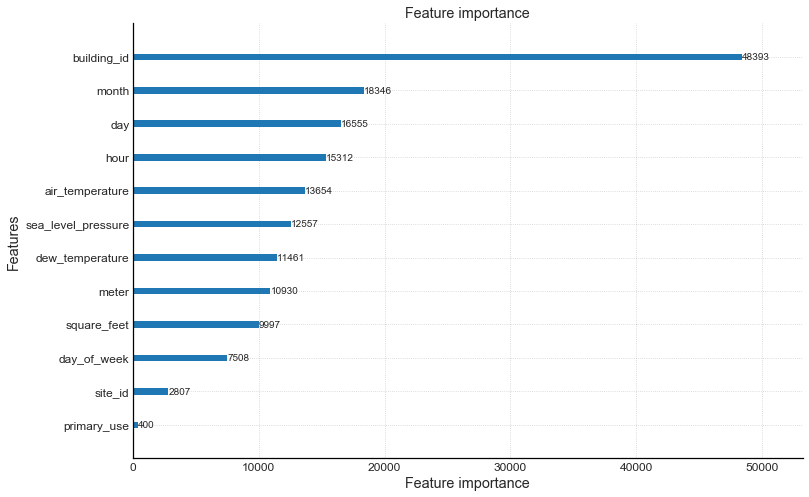
From the figure above, we can conclude that seasonality, in general, is an important predictor of a building’s energy consumption. Seasonality includes variables ‘month’, ‘day’, ‘hour’, and ‘air temperature’. One of the most important features is the building_id which implies that there is something about the building itself that is a great contributing factor to the energy usage. In other words, the variable building_id is a representative of a set of feature space. So, although we have data about the buildings, something still appears to be missing which would further explain the energy usage of that building. Perhaps more data is needed about the building itself to further explains its energy consumption.

Conclusion

Reducing energy usage of a building is important for various reasons including financial and environmental impact. This is a practical problem to solve but also presents unique challenges. The resulting model is relatively accurate, but its results also seem to imply that more data is needed. As discussed earlier, building_id is an interesting predictor since it’s simply an integer. Perhaps it may represent the address of the building and was encoded as an integer for privacy reasons. So, does the address make an important predictor in that case? Do the surrounding buildings affect the energy consumption? These are some of the questions that cannot be answered here but may be answered with additional data.

Further Work

There are numerous other methods which may improve the model further. One such method is build multiple models, one model for each meter type, electric, chilled water, hot water, and steam. Building a model for each meter may lower the error if the model is better able to capture the seasonal trend that exists for meters such as steam and chilled water. The resulting four models may be a bit more difficult to evaluate as opposed to having a single model. Each model may have its own set of hyper-parameters to optimize and must be cross validated. However, it is possible that the error will be reduced further with these four models. Another method is to build a model each site. This would result in creating 16 individual models and again would provide its own set of difficulties that come with evaluating multiple models.

Besides building models, we can try to improve the feature engineering portion of the project. The features added were simply extracted from the timestamp. Perhaps transforming the existing features or adding more useful features may reduce the error even further. Transformations such as scaling is typically not required for tree-based models, but it may be worth trying to reduce the error. Also, transforming the target variable using the natural logarithm provided impressive results so it’s also worth experimenting with other transformations of the target or feature variables.

Sources

1. “ASHRAE - Great Energy Predictor III”. Competition Description. https://www.kaggle.com/c/ashrae-energy-prediction
2. “ASHRAE - Great Energy Predictor III”. Data Description. https://www.kaggle.com/c/ashrae-energy-prediction/data
3. “Parameters Tuning - LightGBM”. https://lightgbm.readthedocs.io/en/latest/Parameters-Tuning.html
4. “Optmization in Accuracy”. https://lightgbm.readthedocs.io/en/latest/Features.html#leaf-wise-best-first-tree-growth

See this project on GitHub